SAP closed the Prior Labs deal a couple of weeks ago and put more than a billion euros behind tabular foundation models. Roughly the same week, I was doing a much smaller thing: pointing TabPFN at bank statement lines in a diligence workload and trying to work out whether it should replace the boosted tree we already had.
The answer took longer than expected, mostly because I spent the first two days measuring the wrong variable. I was comparing models. The variable that actually moved was which rows I put in the context window.
What “fit” means when there is no gradient step
A tabular foundation model does not train on your table. TabPFN v2 tokenizes at the cell level and alternates attention two ways, across the features inside a row, then across the rows inside a feature. It was pre-trained on millions of synthetic tables, so by the time it sees yours it has already learned what tabular structure looks like in general. Calling .fit() loads your labelled examples into a context. Calling .predict() runs one forward pass with those examples sitting in front of the query rows.
Two things follow from that, and they are both operationally annoying.
The attention is quadratic in the number of cells, so the context has a hard ceiling. v2 tops out around ten thousand samples, five hundred features, ten classes. The 2.5 release pushed the row and feature ceilings out a long way, roughly fifty thousand rows and two thousand features, and moved the class ceiling much less. The second thing is that the model is permutation invariant on both axes, which sounds like a nice property and mostly is, but it also means row order carries no information you can use. You cannot sequence your way out of the cap. You can only choose.
So the engineering question stops being “which model” and becomes “which ten thousand rows, chosen how, per batch.”
That is retrieval. Same shape as chunking for RAG, same failure modes, and just as under-measured.
The ledger does not fit, obviously
The workload: statement lines coming out of extraction, needing a chart-of-accounts code before anyone can build a quality-of-earnings view on top. The history behind it is millions of lines across engagements, tens of thousands of distinct counterparties, and a label space in the hundreds once you go past the top level.
Everything about that is over the ceiling. Rows, cardinality, classes.
Classes go first, and the fix is structural, not clever. Predict a coarse bucket, then a second model inside the bucket. Ten-ish labels at each level, two forward passes, done. You pay for it with a hierarchy to maintain and a bad first hop being unrecoverable, the same tradeoff any coarse-to-fine classifier makes.
Cardinality goes second, and counterparty strings get target statistics rather than five hundred one-hot columns. Rows are the interesting one.
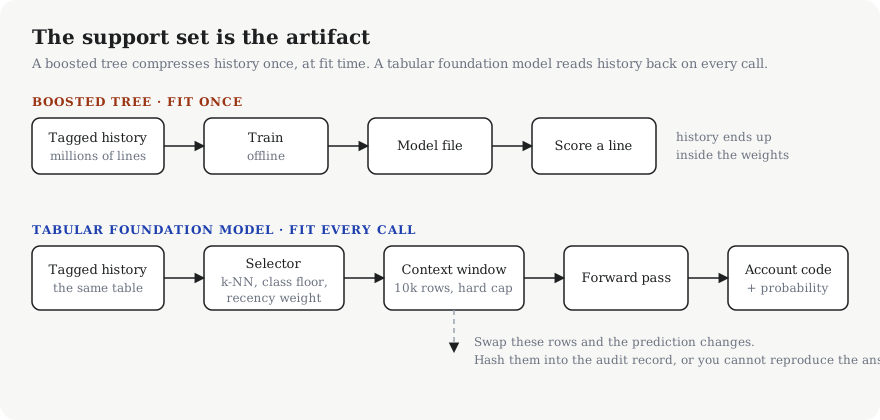 The tree bakes history into weights once. The foundation model reads history back on every call, through a selector you wrote, which makes that selector a production component with a version and a blast radius.
The pool is a query, not a file
Before anything gets selected there has to be a pool, and in our case the pool is a Postgres query that runs per engagement. Three of the conditions in it are load-bearing.
-- Support pool for one engagement. The isolation filter lives in the query,
-- not in a pandas mask afterwards. A row that reaches the context window has
-- already influenced the answer.
select  t.transaction_id,
        t.value_date,
        t.amount_minor,
        t.direction,                        -- 'debit' | 'credit'
        t.counterparty_raw,
        t.description_raw,
        g.account_code,
        (current_date - t.value_date)::int as age_days
from        extraction_transactions t
join        import_sessions   i on i.session_id = t.session_id
join        transaction_tags  g on g.transaction_id = t.transaction_id
where       i.engagement_id = :engagement_id
  and       i.tier          = 'prod'        -- staging lines are not evidence
  and       g.status        = 'accepted'    -- a reviewer signed this, not a model
  and       g.tagged_at     < :as_of        -- nothing tagged after the batch we score
order by    t.value_date desc
limit       200000;                         -- the selector narrows this to the window
status = 'accepted' is the one I would put in bold if I could. Tags the model produced itself are not eligible. Let them in and the context fills with the model’s own past guesses, it hardens on the codes it already favours, and the review queue stops surfacing the cases you needed a human for. In tree terms that is training on your own predictions. In context terms it arrives faster, since there is no retrain step to catch it at.
tagged_at < :as_of is the temporal cut. Reopened engagements make it very easy to hand the model rows a reviewer coded last month while scoring a batch from six months earlier, which gives you a lovely holdout number and a system that cannot repeat it.
Then the encoding, which is where a statement line stops being text.
def encode(df, stats):
    # Statement lines are one number and a lot of string. The number is easy.
    x = pd.DataFrame(index=df.index)
    x["amount_log"]   = np.log1p(df.amount_minor.abs() / 100)
    x["is_credit"]    = (df.direction == "credit").astype(int)
    x["day_of_month"] = df.value_date.dt.day
    x["is_round"]     = (df.amount_minor % 100_000 == 0).astype(int)   # round = transfer, usually
    x["month_span"]   = df.counterparty_norm.map(stats.month_span).fillna(0)

    # Counterparty is the signal and it is high cardinality, so it comes in as
    # a smoothed P(code | counterparty) computed on the support pool ONLY.
    # Compute it across the query rows and you have handed the model the label
    # it is supposed to be predicting.
    x["cp_prior"]     = df.counterparty_norm.map(stats.cp_prior).fillna(stats.global_prior)
    return x.fillna(0.0)
That leaves me with a few dozen columns, nowhere near the five hundred feature ceiling. The row ceiling is the one that bites.
Four ways to pick, and only one of them is free
There’s four strategies worth putting head to head against a fixed holdout.
Uniform sample, the default in every tutorial, which spends most of the window on lines that look nothing like what you are scoring. Stratified by label, better because rare account codes stop vanishing, still blind to the query. Per-query k-NN in encoded feature space, pulling the nearest tagged lines per batch and deduping the union. Expensive, needs a warm index, and it was the one that moved the metric. Chunked ensemble, splitting the pool into context-sized chunks and averaging the logits across forward passes, which is the Chunked TabPFN approach and does recover accuracy on big pools. It also multiplies the inference bill by the chunk count, so it died on cost before it got to a quality argument.
The selector I kept is k-NN with a floor per class and a recency weight, because in diligence the vendor mix from two years ago is not evidence about this year.
from sklearn.neighbors import NearestNeighbors
import numpy as np

# Runs before every scoring batch. There is no equivalent file in the
# XGBoost version of this pipeline, which is the whole difference.
def build_support(pool, queries, cap=9000, floor=40, half_life=120):
    # pool    : previously accepted lines we are allowed to reuse here
    # queries : the unlabelled batch about to be classified
    # Order is irrelevant to the model (permutation invariant on both axes),
    # so this is a "which rows" problem and never a "what order" problem.
    w = 0.5 ** (pool.age_days.to_numpy() / half_life)

    knn = NearestNeighbors(n_neighbors=64, metric="euclidean")
    knn.fit(pool.encoded)          # standardised numerics + target-encoded counterparty
    _, idx = knn.kneighbors(queries.encoded)

    picked, seen = [], set()
    for row in idx:                # nearest first, deduped across the batch
        for i in row:
            if i not in seen:
                seen.add(i)
                picked.append(i)

    # A class the model never sees in context is a class it cannot predict.
    # This loop is slow and I do not care, it runs once per batch and it buys
    # back the long tail for about three percent of the window.
    for label, group in pool.groupby("account_code").indices.items():
        have = sum(1 for i in picked if pool.account_code.iat[i] == label)
        if have < floor:
            extra = [i for i in sorted(group, key=lambda i: -w[i]) if i not in seen]
            picked.extend(extra[: floor - have])

    return pool.iloc[picked[:cap]]
Measure the spread, not the mean
The number nobody publishes is variance across support draws, and it is the number that decided this for me.
Fix the holdout. Resample the support set twenty times with different seeds. Score each. Report the 5th and 95th percentile of macro F1, not the average.
scores = []
for seed in range(20):
    sup = build_support(pool.sample(frac=1.0, random_state=seed), batch)
    clf = TabPFNClassifier(device="cuda")
    clf.fit(sup[FEATURES], sup.account_code)
    scores.append(macro_f1(holdout.account_code, clf.predict(holdout[FEATURES])))

print(np.percentile(scores, [5, 50, 95]))
On our data that spread, from one support draw to another with the model held constant, was wider than the gap between TabPFN and a tuned XGBoost on identical features. Which reframes every benchmark post you have read this month. If swapping ten thousand rows moves the metric more than swapping the model does, then “foundation model beats gradient boosting” is a statement about somebody’s sampler, not about the models.
Going from uniform to k-NN bought more than any model swap I tried. The tree did not care at all, it had already seen the whole pool at fit time, so the gain was real but it was a gain against the foundation model’s own weaker configuration.
Calibration was where I changed my mind about deployment. Raw, the foundation model was better calibrated than the raw tree, expected calibration error noticeably lower before any post-processing. The catch is that its calibration moves with the support set. A stable miscalibration you fit isotonic regression to once and forget. One that drifts whenever the selector picks differently is worse than a predictable bias, because a probability threshold is what decides whether a human ever looks at the line.
What this does to reproducibility
Diligence work gets re-opened. Someone asks in November why a line was coded the way it was in July, and “the model said so” does not survive the follow-up when the model is fixed pre-trained weights plus nine thousand rows chosen by a function reading a table that has moved since.
The tree version of this problem is solved by pinning a model file. The foundation model version needs you to pin the support set.
def provenance(support, selector_cfg, weights_id):
    # Written next to every classification. Reproducing a July coding decision
    # in November means replaying these exact rows, so pool rows get soft
    # deleted and never hard deleted, otherwise the hash points at nothing.
    ids = "|".join(sorted(support.transaction_id.astype(str)))
    return {
        "weights_id":   weights_id,                 # pre-trained, fixed, boring
        "selector":     selector_cfg,               # k, floor, half_life, encoder version
        "support_sha":  hashlib.sha256(ids.encode()).hexdigest(),
        "support_n":    int(len(support)),
        "as_of":        selector_cfg["as_of"],
    }
It is not free. The hash lives beside every prediction, the pool rows have to stay retrievable, and a reviewer retagging an old line changes what a replay would produce unless you version the tags too. Without it there is no reproducing anything, so it ships.
The multi-tenant version of the same fact is sharper. Support rows are the model. If a row from one engagement lands in another engagement’s context window, that is not a feature, that is a client’s data influencing a different client’s output. Which is why the engagement filter sits in the SQL above and not in a dataframe mask three functions later.
Where I landed
The tree is still scoring the bulk of the volume. It is faster by orders of magnitude per line, a tree traversal against a GPU forward pass over a ten thousand row context is not a close race, and it holds the long tail of account codes better once there are enough labels to learn from.
The foundation model won the cold start. A new engagement with a few hundred accepted lines and no history is precisely where a boosted tree has nothing to work with, and where in-context learning is genuinely good. So it runs first, the tree takes over once the labelled pool for that engagement crosses a threshold, and the selector is the piece I actually spend my time on.
The threshold itself is a number I picked by eye, somewhere in the low hundreds of accepted lines, and I have not found a principled way to set it. It is the open item on my desk.